Doug Was Right: I Swapped In The MoE, And The Concurrency Math Changed
Last post I measured the concurrency ceiling on a 27B dense model and closed with a promise. Doug Ware, who builds applied AI systems, had handed me the one caveat I did not test: a dense model is the hard case, and a mixture-of-experts model with only about 3B active parameters per token should leave real headroom for a second slot to pay off. So I ran the exact same 36-load matrix on an MLX MoE, changed one variable, and let the numbers settle it. The dense model flatlines. The MoE keeps climbing. And at 8 concurrent agents the dense model makes you wait 32 seconds for a first token while the MoE answers in under 1.
Two days ago I posted 36 barrier-synchronized loads against 1 local model and let the numbers answer a question Reddit handed me. That post ended with a promise. A reader named Doug Ware, who builds applied AI systems for a living, had replied with the one caveat I had not tested, and I said out loud that measuring it was the next thing I would do. This is that measurement. I did not wait, I did not hand-wave it, and I kept every honest asterisk in.
Here is the short version before the charts. Doug was right. On the dense model, a second concurrent agent barely helps and a fourth helps not at all. Swap in the mixture-of-experts model he pointed me toward, change nothing else, and the wall moves. The total throughput keeps climbing all the way to 8 agents, and the wait for a first token stays under 1 second where the dense model climbed past 30.
The Housekeeping Note
If you are new here, last month a post of mine got called AI slop on Reddit. My full answer, and the standard I hold my own writing to, lives on its own page: On Slop, And Who Gets To Call It That. Every number below was measured on my own hardware with a load driver I wrote. Nothing here is estimated, and the run matrix is on disk next to last week’s. That is the whole point of doing it this way.
The Caveat I Was Handed
Credit where it is due, because this entire post is Doug Ware’s idea rendered in ink.
In the last post I ran everything on a 27B DENSE model, which is close to the worst case for this exact ceiling. In a dense model every single decoded token re-reads all 27B of weights out of one shared memory pool. Decode is memory-bandwidth-bound, so 2 decode streams do not add a second lane of speed, they split the 1 lane you already had.
Doug replied with the fix. He prefers a 35B-A3B mixture-of-experts model over a 27B dense one for daily use, precisely because it leaves him enough tokens per second to make parallel slots worthwhile. A mixture-of-experts model only activates a small fraction of its parameters for each token. So it re-reads a fraction of the memory per token, which means less memory traffic per token, which means real headroom left over for a second, third, and eighth stream to actually use. He also mentioned something that maps straight onto the agent stall I showed last time: in his own tooling he added switches to turn OFF the parallel behavior that cloud providers leave on by default, because on dense models and slower hardware that default hurts.
So I went and measured his claim the only honest way, which is to change exactly 1 thing.
The Rig, And The One Variable I Changed
Same load driver as last time, because it is the only fair one. A human cannot start 2 agents at the same instant, so any hand-run test measures my launch timing, not concurrency. The driver holds every request at a barrier, releases all of them at the same microsecond, fires them at a live mlx_lm.server, and records aggregate throughput, per-agent decode rate, and time to first token. I ran the identical 36-load matrix from the last post: a concurrency sweep, a prefill-versus-decode split, and a prompt-length sweep, each repeated so I report medians instead of trusting one noisy run.
The only thing I changed between the two runs is the model, and I deliberately held the serving stack constant so the comparison is clean:
- Dense, last week: Qwen 3.8 at 27B, four-bit, on MLX. Every token reads all 27B of weights.
- MoE, this week: Qwen3-30B-A3B, four-bit, on MLX. About 30B total parameters, but only about 3B active per token.
Both served by the same mlx_lm.server, same box, same MLX, both warm before I measured. I did not switch to a different serving engine, because that would change 2 variables at once and confound the result. This is dense-versus-MoE and nothing else.
Finding 1: The Dense Model Flatlines. The MoE Keeps Climbing.
I released 1, then 2, then 4, then 8 identical requests at the same instant, against each model, and watched the total throughput.

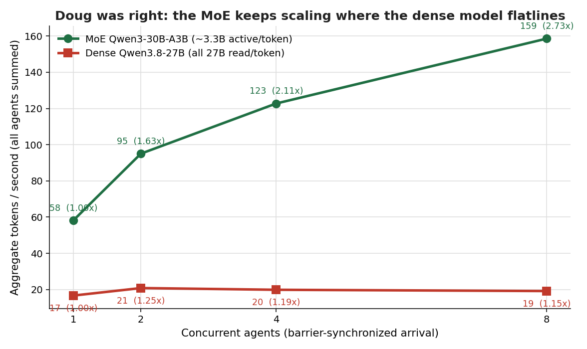
The red line is the dense model from last week. The green line is the MoE. The gap is the whole post.
| Concurrent agents | Dense aggregate tok/s | MoE aggregate tok/s | Dense first-token wait | MoE first-token wait |
|---|---|---|---|---|
| 1 | 16.6 | 58.1 | 0.5s | 0.3s |
| 2 | 20.8 | 95.0 | 3.5s | 0.3s |
| 4 | 19.9 | 122.8 | 10.7s | 0.5s |
| 8 | 19.1 | 158.6 | 32.2s | 0.8s |
On the dense model, going from 1 agent to 2 bought about a quarter more total throughput, and going from 2 to 8 bought nothing. The aggregate sat pinned near 20 tokens per second no matter how many agents I added. That is the ceiling from last week.
On the MoE, the total throughput climbed the entire way: 58, then 95, then 123, then 159 tokens per second. At 8 agents the MoE is moving more than 8 times the tokens the dense model could, and it was still rising when I stopped. The second slot pays off, and so does the fourth, and so does the eighth. That is Doug’s point, measured.
The first-token column is the part that will change how you actually use these things. On the dense model, an 8th agent waited 32 seconds before it saw a single token, because it was stuck behind everyone else fighting for the one memory bus. On the MoE, that same 8th agent got its first token in under 1 second. If you have ever wondered why a busy local model feels like it froze, that column is the answer, and the MoE mostly makes the feeling go away.
Finding 2: Eight MoE Agents Each Beat One Dense Agent
The total throughput is the pie. This next chart is what any single agent actually feels while the others are running.
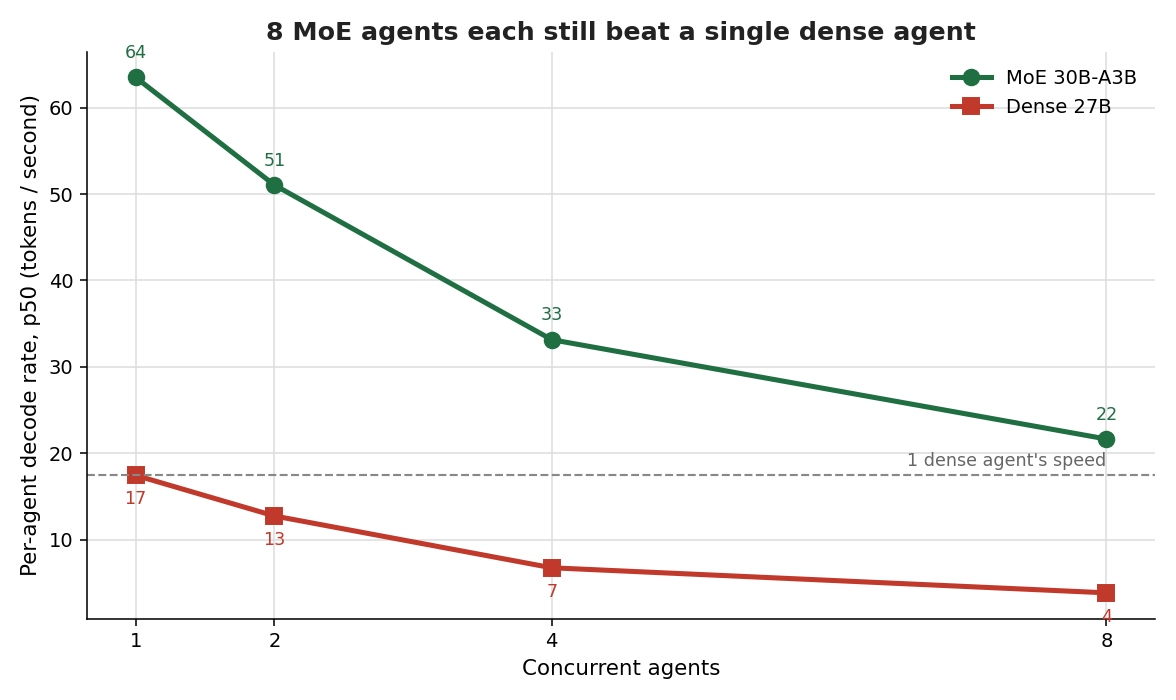
| Concurrent agents | Dense per-agent decode | MoE per-agent decode |
|---|---|---|
| 1 | 17.4 | 63.5 |
| 2 | 12.8 | 51.0 |
| 4 | 6.8 | 33.2 |
| 8 | 3.9 | 21.6 |
Both models slow down per agent as you pile on load, because the bandwidth budget is still shared. That part does not go away, and I am not going to pretend it does. But look at where each one starts and ends. A single dense agent runs at about 17 tokens per second. Eight MoE agents, all running at once, each still decode at about 22 tokens per second. That is the headline in one line: on this hardware, 8 concurrent MoE agents each feel faster than 1 lonely dense agent. On the dense model, 8 agents crawl at under 4 tokens per second each.
Finding 3: The Honest Correction, Because I Always Keep One In
Here is the asterisk on my own headline, because measuring is only worth anything if I report the parts that complicate the story too.
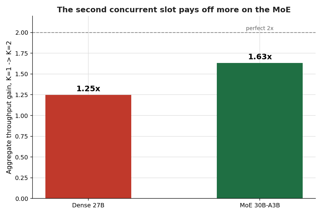
Across the full concurrency sweep the two models look nothing alike, and that is real. But in one specific corner of the matrix, the narrow decode-heavy test at just 2 agents, short prompt and long output, they land close together. The dense model there scaled 1.57 times and the MoE 1.55 times. If I had only run that one cell, I would have concluded the MoE does not help, which is exactly the trap of a single measurement.
The difference only opens up when you look at 2 things the single cell hides. The first is the full sweep out to 8 agents, where the dense model has no room left and the MoE keeps converting concurrency into throughput. The second is absolute speed, because every MoE agent starts about 3 and a half times faster than a dense one, so even the same scaling factor is riding on a much bigger number. So the honest framing is not that the MoE magically doubles where the dense model does not. It is that the dense model hits a hard aggregate ceiling around 20 tokens per second and the MoE has the bandwidth headroom to keep going, while starting far higher. Same shape of scaling in one narrow cell, completely different ceiling everywhere else.
Why This Happens, In One Paragraph
Decode is bound by memory bandwidth, not by compute. The dense model moves all 27B of its parameters out of memory for every single token. The MoE moves only the roughly 3B it activates for that token. Bandwidth is a fixed budget on this machine, so the model that spends less of it per token leaves more of it for the next concurrent stream. That is the entire mechanism. Fewer bytes per token, more room for more tokens, which is precisely what the climbing green line is showing you.
What This Does Not Claim, And What Is Still Next
I want to fence the result honestly.
This measured throughput under concurrency. It did not measure answer quality, which is a completely separate axis, so nothing here says the MoE is a better model for any given task, only that it carries concurrent load far better on this hardware. I also did not mix serving stacks. Both models ran on MLX. I have a much larger MoE sitting on this same machine served by a different engine, and comparing it here would have quietly changed 2 variables at once instead of 1, so that cross-engine question is its own future post.
And 2 of Doug’s threads are still open on my bench. He mentioned switches to turn the default parallel behavior OFF, which is the exact knob that would have saved my stalled agent last week, and he pointed me at a serving-stack change that may finally unlock the speculative decoding I could not turn on before. Both are next. I am going to measure those the same way I measured this, one variable at a time, and show you the matrix. Wait for it.
The Receipt For This Piece
| Signal | This piece of work |
|---|---|
| Where the numbers came from | The same barrier-synchronized load driver I wrote, firing at the live server |
| Human-launch bias in the measurement | Removed by design, all requests released at the same instant |
| Variables changed between the two runs | 1, the model, dense to MoE, serving stack held constant |
| Loads behind the charts | 36, the identical matrix from the last post, re-run on the MoE |
| Repeats per point | 2 to 3, reported as medians |
| Whose hypothesis this tested | Doug Ware’s, credited by name |
| Correction kept in against my own headline | 1, the narrow decode-heavy cell where both models scale alike |
| Threads still open and named | 2, the parallel-off switch and the speculative-decoding serving change |
| Numbers estimated or rounded from vibes | 0 |
| Is the test rig reproducible | Yes, the driver, prompts, and both run matrices are on disk |
The full standard behind this, and why I attach a receipt to work like this, is on the slop page.